A first look at the bitcoin time series

time-series bitcoin

Posted March 23, 2024 by

---

Intention

This post will be the start of a series of Bitcoin-related articles.

Why Bitcoin? We all know that it is a time series, which seems to be ultimately unpredictable, just like the stock market or similar systems.

But it is precisely this feature that makes it the ultimate challenge. We'll try our luck with a number of current MLP methods and put our own spin on them.

In this first post we will analyse the properties of the bitcoin time series with a couple of different statistical tools.

Source

You can find the jupyter-notebook, which forms the basis of this blog post here.

First look at the bitcoin time series

So, let's have a very first look at the data!

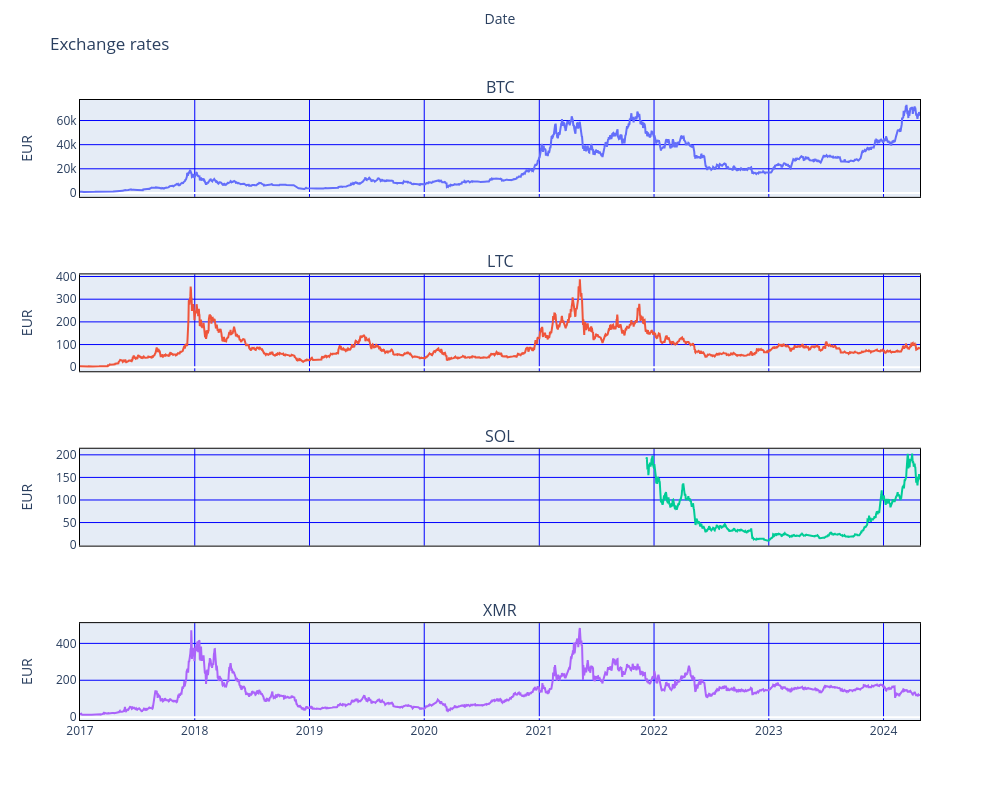
Below are the last few years of Bitcoin (btc) and some alternative coins against the Euro (EUR). It is clear that a coupling between the betcoin and its siblings exists, but it seems to be variabel, depending on the time period.

In particular the latest extended high of the Bitcoin is duplicated in the course history of the Solana (SOL), but neither Litecoin (LTC) nor Monero (XMR) show this trend. Both coins remain approximately constant.

The reason is probably that the coins serve different purposes: while both LTC and XMR serve real-world purposes as actual means of payment, both BTC and SOL remain investment objects. The latest Bitcoin high is driven by the SECs decision to approve trading in Bitcoin funds (ETFs) on the stock exchange. Interestingly this is also mirrored by the course high of the Solana.

Scaling and Fourier transform

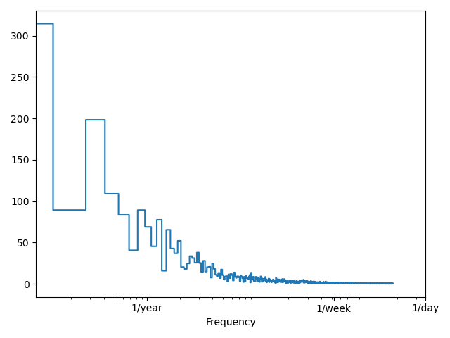
Before applying the Fourier transfom, we scaled the data with sklearns MinMaxScaler and subtracted the average, in order to minimize the effect of steady state components. The Fourier transform can help to identify seasonal periods.

Interestingly, there is a huge peak at the 0-frequency, indicating that there is a strong DC-component (a significant steady-state) in the data. Since we cleaned the data as described above before applying the transform, it can be hypothesized that the DC component is due to the strong general upward trend of the exchange rate over the years. Maybe it is due to the fact that the time series is not stationary? We will check for stationarity later.

More interesting is the peak at the bi-montly frequency. Later on we will use this time window in our prediction model. However, it is not clear why this peak is so prominent and whether or not it is of any use for our prediction.

Is the btc-course a randomwalk?

Now let's determine, whether the bitcoin data is a random walk. We will use the Augmented Dickey-Fuller test to find out.

What is a random walk?

A random walk is a time series, whose first derivative is stationary (meaning that its statistical properties like mean or variance won't change over time) and uncorrelated.

Stationarity of first derivative

We can test the stationarity of the first derivative with the so-called Augmented Dickey-Fuller test, which calculates - among other statistics - the so-called p-value. If p is < 0.05, than it can be assumed that this is a stationary process. Hence, if the p-value of the first derivative is < 0.05, the original time series is a random walk!

from statsmodels.graphics.tsaplots import plot_acf
from statsmodels.tsa.stattools import adfuller

# differentiate the btc-data
df_BTC_diff = np.diff(data.df_BTC['open'], n=1)

adfuller_result = adfuller(df_BTC_diff)

print (f'p-value (should be < 0.05 in order to be a stationary process): {adfuller_result[1]}')

[out] p-value (should be < 0.05 in order to be a stationary process): 4.738918048867276e-13

Autocorellation of the first derivative

plot_acf(df_BTC_diff, lags=20)

plt.ylim(-0.2, 1.2)
plt.tight_layout()

Autocorrelation plot

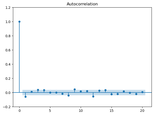
Interpretation: The blue shaded band shows the bandwidth, in which the correlation of a time step with its lagged version is not significantly different from 0. Unsurprisingly, the plot shows an autocorrelation of 1, in other words: a time step correlates with itself. For all other lags between timesteps, the correlation is not significantly different from 0.

Result

According to both tests, Augmented Dickey-Fuller test, the bitcoin data is a random walk!

• The Augmented Dickey-Fuller test results in a p-value significantly smaller than 0.05, indicating stationarity of the first difference.

• The autocorrelation plot reveals, that the correlation between time steps is smaller than or very close to 5 %, which is statistically strong significance that there is no autocorrelation.

Predicting a random walk by its own previous is not possible. So how do we proceed from here? See next article in this series!